C1 summary

Chapter 1 summary - Algebra and functions

1. You can simplify expressions by collecting like terms.
   
   
2. You can simplify expressions by using rules of indices (powers).
   
   a^m \times a^n = a^{m+n}
   a^m \div a^n = a^{m-n}
   a^{-m} = {1\over a^m}
   a^{1\over m} = \root m \of a
   a^{n\over m} = \root m \of {a^n}
   (a^m)^n = a^{mn}
   a^0 = 1
   
   
3. You can expand an expression by multiplying each term inside the bracket by the term outside.
   
   
4. Factorising expressions is the opposite of expanding expressions.
   
   
5. A quadratic expression has the form ax^2 + bx + c , where a, b, c are constants and a \not= 0 .
   
   
6. x^2 - y^2 = (x+y)(x-y)
   
   This is called a difference of squares.
   
   
7. You can write a number exactly using surds.
   
   
8. The square root of a prime number is a surd.
   
   
9. You can manipulate surds using the rules:
   
   \sqrt {ab} = \sqrt {a} \times \sqrt {b}
   \displaystyle \sqrt {a\over b} = {\sqrt {a}\over \sqrt {b}}
   
   
10. The rules to rationalise surds are:
    
    
    • Fractions in the form \displaystyle {1\over \sqrt {a}} , multiply the top and bottom by \sqrt {a} .
    • Fractions in the form \displaystyle {1\over \sqrt {a+\sqrt {b}}} , multiply the top and bottom by a - \sqrt {b} .
    • Fractions in the form \displaystyle {1\over \sqrt {a-\sqrt {b}}} , multiply the top and bottom by a + \sqrt {b} .

Chapter 2 summary - Quadratic functions

1. The general form of a quadratic equation is y =ax^2 + bx + c where a, b, c are constants and a \not= 0 .
   
   
2. Quadratic equations can be solved by:
   
   
   • Factorisation.
   • Completing the square:
     
     \displaystyle x^2 + bx = \left(x+{b\over 2}\right)^2 - \left({b\over 2}\right)^2
     
     
   • Using the formula
     
     \displaystyle x = {-b \pm \sqrt {b^2-4ac}\over 2a}
   
   
3. A quadratic equation has two solutions, which may be equal.
   
   
4. To sketch a quadratic graph:
   
   
   • Decide on the shape:
     
     a > 0 \quad \cup
     a < 0 \quad \cap
     
     
   • Work out the x-axis and y-axis crossing points.
   • Check the general shape by considering the discriminant b^2-4ac .

Chapter 3 summary - Equations and inequalities

1. You can solve linear simultaneous equations by elimination or substitution.
   
   
2. You can use the substitution method to solve simultaneous equations, where one equation is linear and the other is quadratic. You usually start by finding an expression for x or y from the linear equation.
   
   
3. When you multiply or divide an inequality by a negative number, you need to change the inequality sign to its opposite.
   
   
4. To solve a quadratic inequality you
   
   
   • solve the corresponding quadratic equation, then
   • sketch the graph of the quadratic function, then
   • use your sketch to find the required set of values.

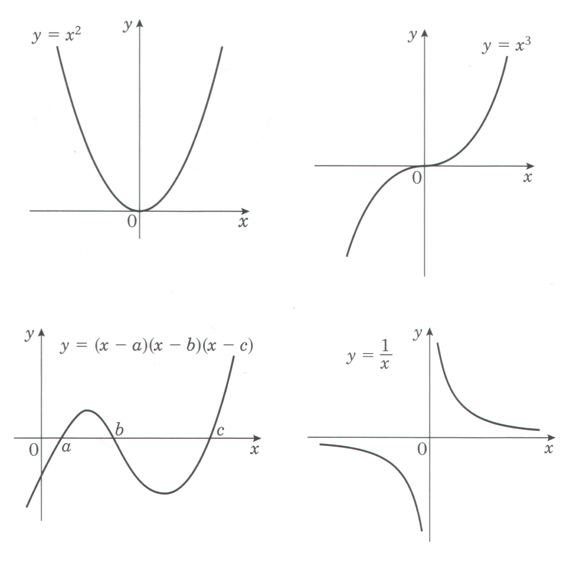
Chapter 4 summary - Sketching curves

1. You should know the shapes of the following basic curves.
   
   
2. Transformations:
   
   f(x+a) is a translation of -a in the x-direction.
   f(x) + a is a translation of +a in the y-direction.
   f(ax) is a sketch of \displaystyle {1\over a} in the x-direction \Bigg( multiply x-coordinates by \displaystyle {1\over a} \Bigg) .
   af(x) is a sketch of a in the y-direction (multiply y-coordinates by a).

Chapter 5 summary - Coordinate geometry in the (x,y) plane

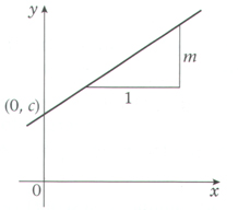
In the general form y = mx + c , where m is the gradient and (0,c) is the intercept on the y-axis. In the general form ax + by + c = 0 , where a, b and c are integers.
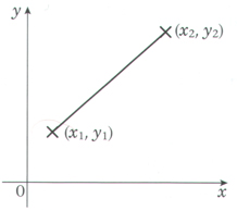
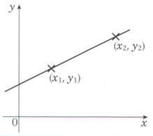
You can work out the gradient m of the line joining the point with coordinates (x_1,y_1) to the point with coordinates (x_2,y_2) by using the formula \displaystyle m = {y_2 - y_1\over x_2 - x_1}
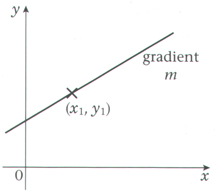
You can find the equation of a line with gradient m that passes through the point with coordinates (x_1, y_1) by using the formula y - y_1 = m(x - x_1)
You can find the equation of the line that passes through the points with coordinates (x_1,y_1) and (x_2,y_2) by using the formula \displaystyle {y-y_1\over y_2-y_1} = {x - x_1\over x_2 - x_1}
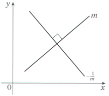
If a line has a gradient m, a line perpendicular to it has a gradient of \displaystyle {-1\over m}.
If two lines are perpendicular, the product of their gradients is -1.

Chapter 6 summary - Sequences and series

1. A series of numbers following a set rule is called a sequence.
   
   3, 7, 11, 15, 19, ... is an example of a sequence.
   
   
2. Each number in a sequence is called a term.
   
   
3. The nth term of a sequence is sometimes called the general term.
   
   
4. A sequence can be expressed as a formula for the nth term. For example the formula U_n = 4n+1 produces the sequence 5, 9, 13, 17, ... by replacing n with 1, 2, 3, 4, etc. in 4n + 1.
   
   
5. A sequence can be expressed by a recurrence relationship. For example the same sequence 5, 9, 13, 17, ... can be formed from U_{n+1} = U_n + 4, U_1=5. (U_1 must be given.)
   
   
6. A recurrence relationship of the form
   
   U_{k+1}=U_k + n, k \geq 1 \quad n \in \unicode{x2124}
   
   is called an arithmetic sequence.
   
   
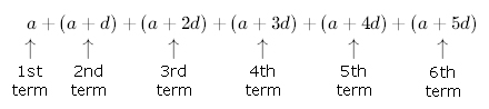
7. All arithmetic sequences can be put in the form
   
   
   
   
8. The nth term of an arithmetic series is a+(n-1)d, where a is the first term and d is the common difference.
   
   
9. The formula for the sum of an arithmetic series is
   
   \displaystyle S_n = {n\over 2}[2a+(n-1)d]
   
   or \displaystyle S_n = {n\over 2}(a+L)
   
   where a is the first term, d is the common difference, n is the number of terms and L is the last term in the series.
   
   
10. You can use \sum to signify 'sum of'. You can use \sum to write series in a more consise way
    
    e.g. \displaystyle \sum^{10}_{r=1}(5+2r)= 7+9+...+25

Chapter 7 summary - Differentiation

1. The gradient of a curve y={\rm f}(x) at a specific point is equal to the gradient of the tangent to the curve at that point.
   
   
2. The gradient of the tangent at any particular point is the rate of change of y with respect to x.
   
   
3. The gradient formula for y={\rm f}(x) is given by the equation gradient = {\rm f}'(x) where {\rm f}'(x) is called the derived function.
   
   
4. If {\rm f}(x)=x^n, then {\rm f}'(x)=nx^{n-1}.
   
   

	Hint: You reduce the power by 1 and the original power multiplies the expression.



5. The gradient of a curve can also be represented by \displaystyle {{\rm d}y\over {\rm d}x} .
   
   
6. \displaystyle {{\rm d}y\over {\rm d}x} is called the derivative of y with respect to x and the process of finding \displaystyle {{\rm d}y\over {\rm d}x} when y is given is called differentiation.
   
   
7. \displaystyle y={\rm f}(x), {{\rm d}y\over {\rm d}x} = {\rm f}'(x)
   
   
8. \displaystyle y=x^n, {{\rm d}y\over {\rm d}x} = nx^{n-1} for all real values of n.
   
   
9. It can also be shown that if x=ax^n where a is a constant, then \displaystyle {{\rm d}y\over {\rm d}x} = nax^{n-1}.
   
   

	Hint: You again reduce the power by 1 and the original power multiplies the expression.



10. If y={\rm f}(x) \pm {\rm g}(x) then \displaystyle {{\rm d}y\over {\rm d}x} = {\rm f}'(x) \pm {\rm g}'(x).
    
    
11. A second order derivative is written as \displaystyle {{\rm d}^2y\over {\rm d}x^2} or {\rm f}''(x), using function notation.
    
    
12. You find the rate of change of a function {\rm f} at a particular point by using {\rm f}'(x) and substituting in the value of x.
    
    
13. The equation of the tangent to the curve y={\rm f}(x) at point A, (a,{\rm f}(a)) is \displaystyle y-{\rm f}(a)=-{1\over {\rm f}'(a)}(x-a).

Chapter 8 summary - Integration

1. If \displaystyle {{\rm d}y\over {\rm d}x}= x^n , then \displaystyle y = {1\over n+1}x^{n+1} + c \quad (n \not= -1) .
   
   
2. If \displaystyle {{\rm d}y\over {\rm d}x}= kx^n , then \displaystyle y = {kx^{n+1}\over n+1} + c \quad (n \not= -1) .
   
   
3. \displaystyle \int x^n{\rm d}x = {x^{n+1}\over n+1} + c \quad (n \not= -1).