C2 summary

Chapter 1 summary - Algebra and functions

1. If {\rm f}(x) is a polynomial and {\rm f}(a)=0, then (x-a) is a factor of {\rm f}(x).
   
   
2. If {\rm f}(x) is a polynomial and \displaystyle {\rm f}\left({b\over a}\right)=0, then (ax-b) is a factor of {\rm f}(x).
   
   
3. If a polynomial {\rm f}(x) is divided by (ax-b) then the remainder is \displaystyle {\rm f}\left({b\over a}\right).

Chapter 2 summary - The sine and cosine rule

1. The sine rule
   
   \displaystyle {a\over \sin A} = {b\over \sin B} = {c\over \sin C}   or   \displaystyle {\sin A\over a} = {\sin B\over b} = {\sin C\over c}
   
   
   
   
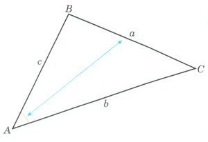
2. You can use the sine rule to find an unknown side in a triangle if you know two angles and length of one of their opposite sides.
   
   
3. You can use the sine rule to find an unknown angle in a triangle if you know the lengths of two sides and one of their opposite angles.
   
   
4. The cosine rule is
   
   a^2 = b^2 + c^2 - 2bc\cos A   or   b^2 = a^2 + c^2 - 2ac\cos B   or   c^2 = a^2 + b^2 - 2ab\cos C
   
   
5. You can use the cosine rule to find an unknown side in a triangle if you know the lengths of two sides and the angle between them.
   
   
6. You can use the cosine rule to find an unknown angle if you know the lengths of all three sides.
   
   
7. You can find an unknown angle using a rearranged form of the cosine rule:
   
   \displaystyle \cos A = {b^2+c^2-a^2\over 2bc} or \displaystyle \cos B = {a^2+c^2-b^2\over 2ac} or \displaystyle \cos C = {a^2+b^2-c^2\over 2ab}
   
   
8. You can find the area of a triangle using the formula
   
   area = {1\over 2}ab\sin C
   
   if you know the length of two sides (a and b) and the value of the angle C between them.

Chapter 3 summary - Exponentials and logarithms

1. A function y=a^x, or {\rm f}(x)=a^x, where a is a constant, is called an exponential function.
   
   
2. \log_a n = x means that a^x = n, where a is called the base of the logarithm.
   
   
3. \log_a 1 = 0
   \log_a a = 1
   
   
4. \log_{10} x is sometimes written as \log x.
   
   
5. The laws of logarithms are
   
   

   \log_a xy = \log_a x + \log_a y	(the multiplication law)
   \displaystyle \log_a \left({x\over y}\right) = \log_a x - \log_a y	(the division law
   \log_a (x)^k = k\log_a x	(the power law)

   
   
   
6. From the power law,
   
   \displaystyle \log_a \left({1\over x}\right) = -\log_a x
   
   
7. You can solve an equation such as a^x=b by first taking logarithms (to base 10) of each side.
   
   
8. The change of base rule for logarithms can be written as \displaystyle \log_a x = {\log_b x\over \log_b a}
   
   
9. From the change of base rule, \displaystyle \log_a b = {1\over \log_b a}

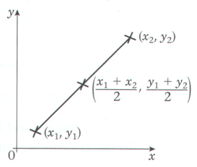
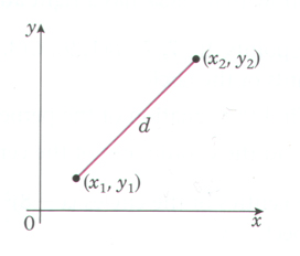
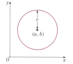
Chapter 4 summary - Coordinate geometry in the (x,y) plane

The mid-point of (x_1,y_1) and (x_2,y_2) is \displaystyle \left({x_1+x_2 \over 2},{y_1+y_2 \over 2}\right).
The distance d between (x_1,y_1) and (x_2,y_2) is d=\sqrt {(x_2-x_1)^2+(y_2-y_1)^2}.
The equation of the circle centre (a,b) radius r is (x-a)^2 + (y-b)^2 = r^2.
A chord is a line that joins two points on the circumference of a circle.
The perpendicular from the centre of a circle to a chord bisects the chord.
The angle in a semicircle is a right angle.
A tangent is a line that meets a circle at one point only.
The angle between a tangent and a radius is 90°.

Chapter 5 summary - The binomial expansion

1. You can use Pascal’s Triangle to multiply out a bracket.
   
   
2. You can use combinations and factional notation to help you expand binomial expressions. For larger indices it is quicker than using Pascal’s Triangle.
   
   
3. n! = n \times (n-1) \times (n-2) \times (n-3) \times ... \times 3 \times 2 \times 1
   
   
4. The number of ways of choosing r items from a group of n items is written ^nC_r or \displaystyle {n\choose r}.
   
   \displaystyle ^3C_2 = {3!\over (3-2)!2!} = {6\over 1 \times 2} = 3
   
   
5. The binomial expansion is
   
   (a+b)^n = {}^nC_0a^n + {}^nC_1a^{n-1}b + {}^nC_2a^{n-2}b^2 + {}^nC_3a^{n-3}b^3 + ... + {}^nC_nb^n
   
   or \displaystyle {n\choose 0}a^n + {n\choose 1}a^{n-1}b + {n\choose 2}a^{n-2}b^2 + {n\choose 3}a^{n-3}b^3 + ... + {n\choose n}b^n
   
   
6. Similarly,
   
   (a+bx)^n = {}^nC_0a^n + {}^nC_1a^{n-1}bx + {}^nC_2a^{n-2}b^2x^2 + {}^nC_3a^{n-3}b^3x^3 + ... + {}^nC_nb^nx^n
   
   or \displaystyle {n\choose 0}a^n + {n\choose 1}a^{n-1}bx + {n\choose 2}a^{n-2}b^2x^2 + {n\choose 3}a^{n-3}b^3x^3 + ... + {n\choose n}b^nx^n
   
   
7. \displaystyle (1+x)^n = 1 + nx + {n(n-1)\over 2!}x^2 + {n(n-1)(n-2)\over 3!}x^3 + {n(n-1)(n-2)(n-3)\over 4!}x^4 + ...

Chapter 6 summary - Radian measure and its applications

If the arc AB has length r, then \angle AOB is 1 radian (1c or 1 rad).
A radian is the angle subtended at the centre of a circle by an arc whose length is equal to that of the radius of the circle. 1 radian \displaystyle = {180^\circ \over \pi}.
The length of an arc of a circle is l=r\theta.
The area of a sector is A={1\over 2}r^2\theta.
The area of a segment in a circle is A={1\over 2}r^2(\theta-\sin \theta).

Chapter 7 summary - Geometric sequences and series

1. In a geometric series you get from one term to the next by multiplying by a constant called the common ratio.
   
   
2. The formula for the nth term = ar^{n-1} where a = first term and r = common ratio.
   
   
3. The formula for the sum to n terms is
   
   \displaystyle S_n = {a(1-r^n) \over 1-r} or \displaystyle S_n = {a(r^n-1) \over r-1}
   
   
4. The sum to infinity exists if |r| < 1 and is \displaystyle S_\infty = {a\over 1-r}

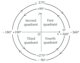
Chapter 8 summary - Graphs of trignometric functions

1. The x-y plane is divided into quadrants:
   
   
   
   

For all values of \theta, the definitions of \sin \theta, \cos \theta and \tan \theta are taken to be \displaystyle \sin \theta = {y \over r} \qquad \cos \theta = {x\over r} \qquad \tan \theta = {y\over x} where x and y are the coordinates of P and r is the radius of the circle.
In the first quadrant, where \theta is acute, All trigonometric functions are positive. In the second quadrant, where \theta is obtuse, only Sine is positive. In the third quadrant, where \theta is reflex, 180^\circ < \theta < 270^\circ, only Tangent is positive. In the fourth quadrant, where \theta is reflex, 270^\circ < \theta < 360^\circ, only Cosine is positive.
The trigonometric ratios of angles equally inclined to the horizontal are related: \sin (180-\theta)^\circ = \sin \theta^\circ \sin (180+\theta)^\circ = -\sin \theta^\circ \sin (360-\theta)^\circ = -\sin \theta^\circ \cos (180-\theta)^\circ = -\cos \theta^\circ \cos (180+\theta)^\circ = -\cos \theta^\circ \cos (360-\theta)^\circ = \cos \theta^\circ \tan (180-\theta)^\circ = -\tan \theta^\circ \tan (180+\theta)^\circ = \tan \theta^\circ \tan (360-\theta)^\circ = -\tan \theta^\circ

5. The trignometric ratios of 30°, 45° and 60° have exact forms, given below:
   
   

   \displaystyle \sin 30^\circ = {1\over 2}	\displaystyle \cos 30^\circ = {\sqrt {3}\over 2}	\displaystyle \tan 30^\circ = {1\over \sqrt {3}} = {\sqrt {3}\over 3}
   \displaystyle \sin 45^\circ = {1\over \sqrt {2}} = {\sqrt {2}\over 2}	\displaystyle \cos 45^\circ = {1\over \sqrt {2}} = {\sqrt {2}\over 2}	\displaystyle \tan 45^\circ = 1
   \displaystyle \sin 60^\circ = {\sqrt {3}\over 2}	\displaystyle \cos 60^\circ = {1\over 2}	\displaystyle \tan 60^\circ = \sqrt {3}

   
   
6. The sine and cosine functions have a period of 360°, (or 2\pi radians).
   
   Periodic properties are
   
   \sin (\theta \pm 360^\circ) = \sin \theta and \cos (\theta \pm 360^\circ) = \cos \theta
   
   respectively.
   
   
7. The tangent function has a period of 180°, (or \pi radians).
   
   Periodic properties is \tan (\theta \pm 180^\circ) = \tan \theta
   
   
8. Other useful properties are
   
   \sin (-\theta) = -\sin \theta; \cos (-\theta) = \cos \theta; \tan (-\theta) = -\tan \theta
   \sin (90^\circ-\theta) = \cos \theta; \cos (90^\circ-\theta) = \sin \theta
   
   
   

Chapter 9 summary - Differentiation

1. For an increasing function {\rm f}(x) in the interval (a, b), {\rm f}'(x)>0 in the interval a \leq x \leq b.
   
   
2. For a decreasing function {\rm f}(x) in the interval (a, b), {\rm f}'(x)<0 in the interval a \leq x \leq b.
   
   
3. The points where {\rm f}(x) stops increasing and begins to decrease are called maximum points.
   
   
4. The points where {\rm f}(x) stops decreasing and begins to increase are called minimum points.
   
   
5. A point of inflexion is a point where the gradient is at a maximum or minimum value in the neighbourhood of the point.
   
   
6. A stationary point is a point of zero gradient. It may be a maximum, a minimum or a point of inflexion.
   
   
7. To find the coordinates of a stationary point find \displaystyle {{\rm d}y\over {\rm d}x}, i.e. {\rm f}'(x), and solve the equation {\rm f}'(x)=0 to find the value, or values, of x and then substitute into y={\rm f}(x) to find the corresponding values of y.
   
   
8. The stationary value of a function is the value of y at the stationary point. You can sometimes use this to find the range of a function.
   
   
9. You may determine the nature of a stationary point by using the second derivative.
   
   
If \displaystyle {{\rm d}y\over {\rm d}x}=0 and \displaystyle {{\rm d}^2y\over {\rm d}x^2}>0, the point is a minimum point.

If \displaystyle {{\rm d}y\over {\rm d}x}=0 and \displaystyle {{\rm d}^2y\over {\rm d}x^2}<0, the point is a maximum point.

If \displaystyle {{\rm d}y\over {\rm d}x}=0 and \displaystyle {{\rm d}^2y\over {\rm d}x^2}=0, the point is either a maximum or a minumum point or a point of inflexion.



	Hint: In this case you need to use the tabular method and consider the gradient on either side of the stationary point.


If \displaystyle {{\rm d}y\over {\rm d}x}=0 and \displaystyle {{\rm d}^2y\over {\rm d}x^2}=0, but \displaystyle {{\rm d}^3y\over {\rm d}x^3}\not= 0, then the point is a point of inflexion.


10. In problems where you need to find the maximum or minimum value of a variable y, first establish a formula for y in terms of x, then differentiate and put the derived function equal to zero to find x and then y.

Chapter 10 summary - Trigonometrical identities and simple equations

1. \displaystyle \tan \theta = {\sin \theta\over \cos \theta} (providing \cos \theta \not= 0, when \tan \theta is not defined)
   
   
2. \sin^2 \theta + \cos^2 \theta = 1
   
   
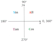
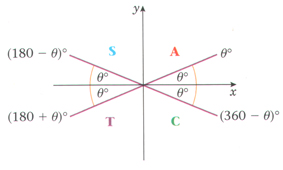
3. A first solution of the equation \sin x = k is your calculator value, \alpha = \sin^{-1} k. A second solution is (180^\circ - \alpha), or (\pi - \alpha) if you are working in radians. Other solutions are found by adding or subtracting multiples of 360° or 2\pi radians.
   
   
4. A first solution of the equation \cos x = k is your calculator value, \alpha = \cos^{-1} k. A second solution is (360^\circ - \alpha), or (2\pi - \alpha) if you are working in radians. Other solutions are found by adding or subtracting multiples of 360° or 2\pi radians.
   
   
5. A first solution of the equation \tan x = k is your calculator value, \alpha = \tan^{-1} k. A second solution is (180^\circ + \alpha), or (\pi + \alpha) if you are working in radians. Other solutions are found by adding or subtracting multiples of 360° or 2\pi radians.

Chapter 11 summary - Integration

1. The definite integral \displaystyle \int_a^b {\rm f}'(x){\rm d}x = {\rm f}(b) - {\rm f}(a).
   
   
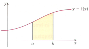
2. The area beneath the curve qith equation y={\rm f}(x) and between the lines x=a and x=b is
   
   Area \displaystyle = \int_a^b {\rm f}(x){\rm d}x
   
   
   
   
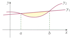
3. The area between a line (equation y_1) and a curve (equation y_2) is given by
   
   Area \displaystyle = \int_a^b (y_1-y_2){\rm d}x
   
   
   
   
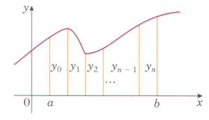
4. Trapezium rule (in the formula booklet):
   
   \displaystyle \int_a^b y {\rm d}x \approx {1\over 2}h [y_0 + 2(y_1 + y_2 + ... + y_{n-1}) + y_n]
   
   where \displaystyle h = {b-a\over n} and y_i = {\rm f}(a+ih).