Algebraic functions can be simplified by cancelling down. To do this the numerators and denominators must by fully factorised first.
If the numberator and denominator contain fractions then you can multiply both by the same number (the lowest common multiple) to create an equivalent fraction.
To multiply fractions, you simply multiply the numerators and multiply the decnominators. If possible cancel down first.
To divide two fractions, multiply the first fraction by the reciprocal of the second fraction.
To add (or subtract) fractions each fraction must have the same denominator. This is done by finding the lowest common multiple of the denominators.
When the numerator hs the same or higher degree than the denominator, you can divide the terms to produce a 'mixed' number fraction. This can be done either by using long division or by using the remainded theorum:
where {\rm Q}(x) is the quotient and is how many times the divisor divides into the function.
Chapter 2 summary - Functions
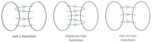
A function is a special mapping such that every element of the domain is mapped to exactly one element in the range.
A one-to-one function is a special function where every element of the domain is mapped to one element in the range.
Many mappings can be made into functions by changing the domain. For example, the mapping 'positive square root' can be changed into the function {\rm f}(x) = \sqrt {x} by having a domain of x \geq 0.
If we combine two or more functions we can create a composite function. The function below is written {\rm fg}(x) as {\rm g} acts on x first, then {\rm f} acts on the result. For example,
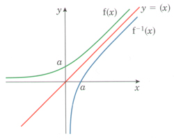
The inverse of a function {\rm f}(x) is written {\rm f}^{-1}(x) and performs the opposite operation(s) to the function. To calculate the inverse function you can change the subject of the formula. For example, the inverse function {\rm g}(x) = 4x - 3 is
\displaystyle {\rm g}^{-1}(x) = {x+3\over 4}
The range of the function is the domain of the inverse function and vice versa.
The graph of {\rm f}^{-1}(x) is a reflection of {\rm f}(x) in the line y=x.
Chapter 3 summary - The exponential and log functions
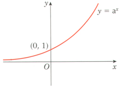
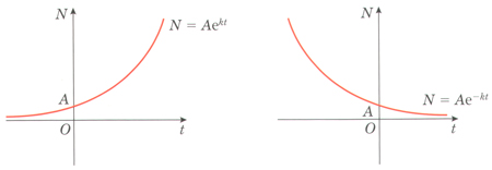
Exponential functions are ones of the form y= a^x.
They all pass through the point (0,1).
The domain is all the real numbers. The range is {\rm f}(x)>0.
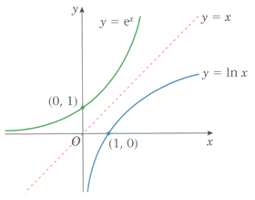
The exponential function y={\rm e}^x (where {\rm e} \approx 2.718) is a special function whose gradient is identical to the function.
The inverse function to {\rm e}^x is \ln x.
The natural log function is a reflection of y={\rm e}^x in the line y=x. It passes through the point (1,0).
The domain is the positive numbers. The range is all the real numbers.
To solve an equation using \ln x or {\rm e}^x you must change the subject of the formula and use the fact that they are inverses of each other.
Growth and decay models are based around the exponential equations
where A and k are positive numbers.
Chapter 4 summary - Numerical methods
If you find an interval in which {\rm f}(x) changes sign, and {\rm f}(x) is continuous in that interval, then the interval must contain a root of the equation {\rm f}(x)=0.
To solve an equation of the form {\rm f}(x)=0 by an iterative method, rearrange {\rm f}(x)=0 into a form x={\rm g}(x) and use the iterative formula x_{n+1}={\rm g}(x_n).
Different rearrangements of the equation {\rm f}(x)=0 give iteration formulae that may lead to different roots of the equation.
If you choose a value x_0=a for the starting value in an iteration formula, and x_0=a is close to a root of the equation {\rm f}(x)=0, then the sequence x_0,x_1, x_2, x_3, x_4 ... does not necessarily converge to that root. In fact it might not converge to a root at all.
Chapter 5 summary - Transforming graphs of functions
The modulus of a number a, written as |a|, is its positive numerical value.
For |a| \geq 0, |a| = a.
For |a| < 0, |a| = -a.
To sketch the graph of y=|{\rm f}(x)|:
Sketch the graph of y={\rm f}(x).
Reflect in the x-axis any parts where {\rm f}(x)<0 (parts below the x-axis).
Delete the parts below the x-axis.
To sketch the graph of y={\rm f}(|x|):
Sketch the graph of y={\rm f}(x) for x \geq 0.
Reflect this in the y-axis.
To solve an equation of the type |{\rm f}(x)| = {\rm g}(x) or |{\rm f}(x)| = |{\rm g}(x)|:
Use a sketch to locate the roots.
Solve algebraically, using -{\rm f}(x) for reflected parts of y={\rm f}(x) and -{\rm g}(x) for reflected parts of y={\rm g}(x).
Basic types of transformation are
{\rm f}(x+a)
a horizontal translation of -a
{\rm f}(x) + a
a vertical translation of +a
{\rm f}(ax)
a horizontal stretch of scale factor \displaystyle {1\over a}
a{\rm f}(x)
a vertical stretch of scale factor a
These may be combined to give, for example, b{\rm f}(x+a), which is a horizontal translation of -a followed by a vertical stretch of scale factor b.
For combinations of transformations, the graph can be built up 'one step at a time', starting from a basic or given curve.
Chapter 6 summary - Trigonometry
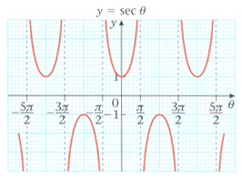
\displaystyle \sec \theta = {1\over \cos \theta} (\sec \theta is undefined when \cos \theta = 0, i.e. at \theta = (2n+1) 90^\circ, n \in \unicode{x2124})
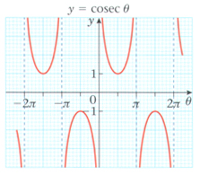
\displaystyle {\rm co}\sec \theta = {1\over \sin \theta} ({\rm co}\sec \theta is undefined when \sin \theta = 0, i.e. at \theta = 180n^\circ, n \in \unicode{x2124})
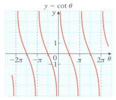
\displaystyle \cot \theta = {1\over \tan \theta} (\cot \theta is undefined when \tan \theta = 0, i.e. at \theta = 180n^\circ, n \in \unicode{x2124})
\cot \theta can also be written as \displaystyle {\cos \theta\over \sin \theta}.
The graphs of \sec \theta, {\rm co}\sec \theta and \cot \theta are
Two further Pythagorean identities identities, derived from \sin^2 \theta + \cos^2 \theta \equiv 1, are
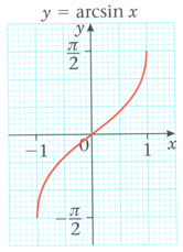
The inverse function of \sin x, \displaystyle -{\pi\over 2} \leq x \leq {\pi \over 2}, is called \arcsin x; it has domain -1 \leq x \leq 1 and range \displaystyle -{\pi\over 2} \leq \arcsin x \leq {\pi \over 2}.
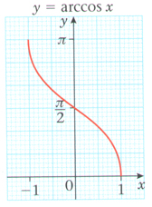
The inverse function of \cos x, 0 \leq x \leq \pi, is called \arccos x; it has domain -1 \leq x \leq 1 and range 0 \leq \arccos x \leq \pi.
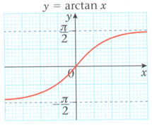
The inverse function of \tan x, \displaystyle -{\pi\over 2} < x < {\pi \over 2}, is called \arctan x; it has domain x \in \Re and range \displaystyle -{\pi\over 2} < \arctan x < {\pi \over 2}.
Chapter 7 summary - Further trigonometric identities and their applications
The addition (or compound angle) formulae are
\sin (A+B) \equiv \sin A\cos B + \cos A\sin B \qquad \qquad \sin(A-B) \equiv \sin A\cos B - \cos A\sin B
\cos (A+B) \equiv \cos A\cos B - \sin A\sin B \qquad \qquad \cos (A-B) \equiv \cos A\cos B + \sin A\sin B
Expressions of the form a\sin \theta + b\cos \theta can be rewritten in terms of a sine only or a cosine only, as follows:
For positive values of a and b, a \sin \theta \pm b\cos \theta \equiv R\sin (\theta \pm \alpha), with R > 0 and 0 < \alpha < 90^\circ, a \cos \theta \pm b\sin \theta \equiv R\cos (\theta \pm \alpha), with R > 0 and 0 < \alpha < 90^\circ
where R\cos \alpha = a, R \sin \alpha = b and R = \sqrt {a^2+b^2}.
Remember you can always use 'the R formula' to solve equations of the form a\cos \theta + b\sin \theta = c, where a, b and c are constants, but if c=0, the equation reduces to the form \tan \theta = k.
Products of sines and/or cosines can be expressed as the sum or difference of sines or cosines, using the formulae:
2\sin A\cos B \equiv \sin (A+B) + \sin (A-B)
2\cos A \cos B \equiv \cos (A+B) + \cos (A-B)
2\cos A\sin B \equiv \sin (A+B) - \sin (A-B)
2\sin A \sin B \equiv -[\cos (A+B) - \cos (A-B)]
Sums or differences of sines or cosines can be expressed as a product of sines and/or cosines, using 'the factor formulae':
You can use the chain rule to differentiate a function of a function:
if y=[{\rm f}(x)]^n then \displaystyle {dy\over dx} = n[{\rm f}(x)]^{n-1}{\rm f}'(x)
if y={\rm f}[{\rm g}(x)] then \displaystyle {dy\over dx} = {\rm f}'[{\rm g}(x)]{\rm g}'(x)
Another form of the chain rule states that \displaystyle {{\rm d}y\over {\rm d}x} = {{\rm d}y\over {\rm d}u} \times {{\rm d}u\over {\rm d}x} where y is a function of u, and u is a function of x.
A particular case of the chain rule is the result \displaystyle {{\rm d}y\over {\rm d}x} = {1\over \left({{\rm d}y\over {\rm d}x}\right)}
You can use the product rule when two functions u(x) and v(x) are multiplied together.
If y=uv then \displaystyle {{\rm d}y\over {\rm d}x} = u{{\rm d}v\over {\rm d}x} + v{{\rm d}u\over {\rm d}x}
You can use the quotient rule when one function u(x) is divided by another function v(x), to form a rational function.
If \displaystyle y = {u\over v} then \displaystyle {{\rm d}y\over {\rm d}x} = {v{{\rm d}u\over {\rm d}x} - u{{\rm d}v\over {\rm d}x}\over v^2}
If y={\rm e}^x then \displaystyle {{\rm d}y\over {\rm d}x} = {\rm e}^x also and if y={\rm e}^{{\rm f}(x)} then \displaystyle {{\rm d}y\over {\rm d}x} = {\rm f}'(x){\rm e}^{{\rm f}(x)}
If y=\ln x then \displaystyle {{\rm d}y\over {\rm d}x} = {1\over x} and if y=\ln [{\rm f}(x)] then \displaystyle {{\rm d}y\over {\rm d}x} = {{\rm f}'(x)\over {\rm f}(x)}
If y=\sin x then \displaystyle {{\rm d}y\over {\rm d}x} = \cos x.
If y=\cos x then \displaystyle {{\rm d}y\over {\rm d}x} = -\sin x.
If y=\tan x then \displaystyle {{\rm d}y\over {\rm d}x} = \sec^2 x.
If y={\rm co}\sec x then \displaystyle {{\rm d}y\over {\rm d}x} = -{\rm co}\sec x\cot x.
If y=\sec x then \displaystyle {{\rm d}y\over {\rm d}x} = \sec x\tan x.
If y=\cot x then \displaystyle {{\rm d}y\over {\rm d}x} = -{\rm co}\sec^2 x.
The chain rule can be used with each of these functions to obtain further results. (See the examples in chapter 8 of the C3 textbook.)