C4 summary

Chapter 1 summary - Partial Fractions

1. An algebraic fraction can be written as a sum of two or more simpler fractions. This technique is called splitting into partial fractions.
   
   
2. An expression with two linear terms in the denominator such as \displaystyle{11\over (x-3)(x+2)} can be split by converting into the form \displaystyle{A\over (x-3)} + {B\over (x+2)} .
   
   
3. An expression with three or more linear terms such as \displaystyle{4\over (x+1)(x-3)(x+4)} can be split by converting into the form \displaystyle{A\over (x+1)} + {B\over (x-3)} + {C\over (x+4)} and so on if there are more terms.
   
   
4. An expression with repeated terms in the denominator such as \displaystyle{6x^2-29x-29\over (x+1)(x-3)^2} can be split by converting into the form \displaystyle{A\over (x+1)} + {B\over (x-3)} + {C\over (x-3)^2} .
   
   
5. An improper fraction is one where the index of the numerator is equal to or higher than the index of the denominator. An improper fraction must be divided first to obtain a number and a proper fraction before you can express it in partial fractions.
   
   
   • For example, \displaystyle{x^2+3x+4\over x^2+3x+2} = 1 + {2\over x^2+3x+2} = 1 + {A\over (x+1)} + {B\over (x+2)} .

Chapter 2 summary - Coordinate geometry in the (x,y) plane

1. To find the cartesian quation of a curve given parametrically you eliminate the parameter t between the parametric equations.
   
   
2. To find the area under a curve given parametrically you use \displaystyle\int y {{\rm d}x\over {\rm d}t}{\rm d}t

Chapter 3 summary - The Binomial Expansion

1. The binomial expansion
   
   \displaystyle (1+x)^n = 1 + nx + {n(n-1)x^2\over 2!} + {n(n-1)(n-2)x^3\over 3!} + ...
   
   can be used to give an exact expression if n is a positive integer, or an approximate expression for any other rational number.
   
   
   • (1+2x)^3 = 1 + 3(2x) + 3 \times 2 {(2x)^2\over 2!} + 3 \times 2 \times 1 {(2x)^3\over 3!} + 3 \times 2 \times 1 \times 0 {(2x)^4\over 4!}
     
     
     \qquad\qquad   = 1 + 6x + 12x^2 + 8x^3
     
     (Expansion is finite and exact.)
     
     
   • \sqrt {(1-x)} = (1-x)^{1\over 2} = 1 + {1\over 2}(-x) + \left({1\over 2}\right)\left({-1\over 2}\right){(-x)^2\over 2!} + \left({1\over 2}\right)\left({-1\over 2}\right)\left({-3\over 2}\right){(-x)^3\over 3!} + ...
     
     
     \qquad\qquad   = 1 - {1\over 2}x - {1\over 8}x^2 - {1\over 16} x^3 + ...
     
     (Expansion is infinite and approximate.)
     
     


2. The expansion \displaystyle (1+x)^n = 1 + nx + n(n-1){x^2\over 2!} + n(n-1)(n-2){x^3\over 3!} + ... , where n is negative or a fraction, is only valid if |x| < 1.
   
   
3. You can adapt the binomial expansion to include expressions of the form (a+bx)^n by simply taking out a common factor of a:
   
   e.g. \displaystyle {1\over (3+4x)} = (3+4x)^{-1} = \left[3\left(1+{4x\over 3}\right)\right]
   \displaystyle \qquad\qquad\qquad\qquad\qquad\qquad = 3^{-1}\left(1+{4x\over 3}\right)^{-1}
   
   
4. You can use knowledge of partial fractions to expand more difficult expressions, e.g.
   
   \displaystyle {7+x\over (3-x)(2+x)} = {2\over(3-x)}+{1\over (2+x)}
   \qquad\qquad\qquad\quad = 2(3-x)^{-1} + (2+x)^{-1}
   \displaystyle \qquad\qquad\qquad\quad = {2\over 3}\left(1-{x\over 3}\right)^{-1} + {1\over 2}\left(1-{x\over 2}\right)^{-1}

Chapter 4 summary - Differentiation

1. When a relation is described by parametric equations:
   
   
   • You differentiate x and y with respect to the parameter t .
   • Then you use the chain rule rearranged into the form \displaystyle {{\rm d}y\over {\rm d}x} = {{\rm d}y\over {\rm d}t} \div {{\rm d}x\over {\rm d}t}.


2. When a relation is described by an implicit equation:
   
   
   • Differentiate each term in turn, using the chain rule and product and quotient rules as appropriate.
     
     
   • \displaystyle {{\rm d}\over {\rm d}x}(y^n) = ny^{n-1}{{\rm d}y\over {\rm d}x}
     
     

   	By the chain rule.

   
   
   • \displaystyle {{\rm d}\over {\rm d}x}(xy) = x{{\rm d}\over {\rm d}x}(y) + y{{\rm d}\over {\rm d}x}(x) = x{{\rm d}y\over {\rm d}x}+y
     
     

   	By the product rule.

   
   
3. In an implicit equation:
   
   
   • Note that when {\rm f}(y) is differentiated with respect to x it becomes \displaystyle {\rm f}'(y){{\rm d}y\over {\rm d}x}.
   • A product term such as {\rm f}(x)\cdot {\rm g}(y) is differentiated by the product rule and becomes \displaystyle {\rm f}(x)\cdot {\rm g}'(y){{\rm d}y\over {\rm d}x} + {\rm g}(y)\cdot {\rm f}'(x)


4. You can differentiate the function {\rm f}(x) = a^x:
   
   
   • If y=a^x , then \displaystyle {{\rm d}y\over {\rm d}x} = a^x \ln a


5. You can use the chain rule once, or several times, to connect the rates of change in a question involving more than two variables.
   
   
6. You can set up simple differential equations from information given in context. This may involve using connected rates of change, or ideas of proportion.

Chapter 5 summary - Vectors

1. A vector is a quantity that has both magnitude and direction.
   
   
2. Vectors that are equal have both the same magnitude and the same direction.
   
   
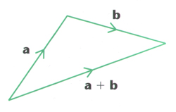
3. Two vectors are added using the 'triangle law'.
   
   
4. Adding the vectors \overrightarrow {PQ} and \overrightarrow {QP} gives the zero vector {\bf 0}.
   
   \Bigl(\overrightarrow {PQ} + \overrightarrow {PQ} = {\bf 0}\Bigr)
   
   
5. The modulus of a vector is another name for its magnitude.
   
   
   • The modulus of the vector {\bf a} is written as |{\bf a}|.
   • The modulus of the vector \overrightarrow {PQ} is written as |\overrightarrow {PQ}|


6. The vector -{\bf a} has the same magnitude as the vector {\bf a} but is in the opposite direction.
   
   
7. Any vector parallel to the vector {\bf a} may be written as \lambda{\bf a}, where \lambda is a non-zero scalar.
   
   
8. {\bf a} - {\bf b} is defined to be {\bf a} + (-{\bf b}).
   
   
9. A unit vector is a vector which has magnitude (or modulus) 1 unit.
   
   
10. If \lambda{\bf a} + \mu{\bf b} = \alpha{\bf a} + \beta{\bf b}, and the non-zero vectors {\bf a} and {\bf b} are not parallel, then \lambda = \alpha and \mu = \beta.
    
    
11. The position vector of a point A is the vector \overrightarrow {OA} , where O is the origin. \overrightarrow {OA} is usually written as vector {\bf a}.
    
    
12. \overrightarrow {AB} = {\bf b} - {\bf a}, where {\bf a} and {\bf b} are the position vectors of A and B respectively.
    
    
13. The vectors {\bf i}, {\bf j} and {\bf k} are unit vectors parallel to the x-axis, the y-axis and the z-axis and in the direction of x increasing, y increasing and z increasing, respectively.
    
    
14. The modulus (or magnitude) of x{\bf i} + y{\bf j} is \sqrt {x^2+y^2}.
    
    
15. The vector x{\bf i} + y{\bf j} + z{\bf k} may be written as a column matrix \pmatrix{x \cr y \cr z}.
    
    
16. The distance from the origin to the point (x,y,z) is \sqrt {x^2 + y^2 + z^2}.
    
    
17. The distance between the points (x_1, y_1, z_1) and (x_2, y_2, z_2) is \sqrt {(x_1 - x_2)^2 + (y_1 - y_2)^2 + (z_1-z_2)^2} .
    
    
18. The modulus (or magnitude) of x{\bf i} + y{\bf j} + z{\bf k} is \sqrt {x^2 + y^2 + z^2}.
    
    
19. The scalar product of two vectors {\bf a} and {\bf b} is written as {\bf a}.{\bf b} , and defined by
    
    {\bf a}.{\bf b} = |{\bf a}||{\bf b}| \cos \theta
    
    where \theta is the angle between {\bf a} and {\bf b} .
    
    
20. If {\bf a} and {\bf b} are the position vectors of the points A and B, then
    
    \displaystyle \cos AOB = {{\bf a}.{\bf b}\over |{\bf a}||{\bf b}|}
    
    
21. The non-zero vectors {\bf a} and {\bf b} are perpendicular if and only if {\bf a}.{\bf b} = 0.
    
    
22. If {\bf a} and {\bf b} are parallel, {\bf a}.{\bf b} = |{\bf a}||{\bf b}|.
    
    
    • In particular, {\bf a}.{\bf a} = |{\bf a}|^2


23. If {\bf a} = a_1{\bf i} + a_2{\bf j} + a_3{\bf k} and {\bf b} = b_1{\bf i} + b_2{\bf j} + b_3{\bf k}
    
    {\bf a}.{\bf b} = \pmatrix{a_1 \cr a_2 \cr a_3} \cdot \pmatrix{b_1 \cr b_2 \cr b_3} = a_1b_1 + a_2b_2 + a_3b_3
    
    
24. A vector equation of a straight line passing through the point A with position vector {\bf a} , and parallel to the vector {\bf b} , is
    
    {\bf r} = {\bf a} + t{\bf b}
    
    where t is a scalar parameter.
    
    
25. A vector equation of a straight line passing through the points C and D, with position vectors {\bf c} and {\bf d} respectively, is
    
    {\bf r} = {\bf c} + t({\bf d}-{\bf c})
    
    where t is a scalar parameter.
    
    
26. The acute angle \theta between two straight lines is given by
    
    \displaystyle \cos \theta = \left|{{\bf a}.{\bf b}\over |{\bf a}||{\bf b}|}\right|
    
    where {\bf a} and {\bf b} are direction vectors of the lines.

Chapter 6 summary - Integration

1. You should be familiar with the following integrals.
   
   \displaystyle \int x^n = {x^{n+1}\over n+1} + C
   \displaystyle \int {\rm e}^x = {\rm e}^x + C
   \displaystyle \int {1\over x} = \ln |x| + C
   \displaystyle \int \cos x = \sin x + C
   \displaystyle \int \sin x = -\cos x + C
   \displaystyle \int \sec^2 x = \tan x + C
   \displaystyle \int {\rm co}\sec\cot x = -{\rm co}\sec x + C
   \displaystyle \int {\rm co}\sec^2 x = -\cot x + C
   \displaystyle \int \sec x\tan x = \sec x + C
   
   
2. Using the chain rule in reverse you can obtain generalisations of the above formulae.
   
   \displaystyle \int f'(ax+b)dx = {1\over a}f(ax+b) + C
   \displaystyle \int (ax+b)^ndx = {1\over a}{(ax+b)^{n+1}\over n+1} + C
   \displaystyle \int {\rm e}^{ax+b}dx = {1\over a}{\rm e}^{ax+b} + C
   \displaystyle \int {1\over (ax+b)}dx = {1\over a} \ln|ax+b| + C
   \displaystyle \int \cos(ax+b)dx = {1\over a}\sin(ax+b) + C
   \displaystyle \int \sin(ax+b)dx = -{1\over a}\cos(ax+b) + C
   \displaystyle \int \sec^2(ax+b)dx = {1\over a}\tan(ax+b) + C
   \displaystyle \int {\rm co}\sec(ax+b)cot(ax+b)dx = -{1\over a}{\rm co}\sec(ax+b) + C
   \displaystyle \int {\rm co}\sec^2(ax+b)dx = -{1\over a}\cot(ax+b) + C
   \displaystyle \int \sec(ax+b)\tan(ax+b)dx = {1\over a}\sec(ax+b) + C
   
   
3. Sometimes trigonometric identities can be useful to help change the expression into one you know how to integrate.
   
   e.g. To integrate \sin^2x or \cos^2x use formula for \cos2x , so
   
   \displaystyle \int \sin^2x{\rm d}x = \int \left({1\over 2}-{1\over 2}\cos2x\right){\rm d}x
   
   
4. You can use partial fractions to integrate expressions of the type \displaystyle {x-5\over (x+1)(x-2)}.
   
   
5. You should remember the following general patterns:
   
   \displaystyle \int {{\rm f}'(x)\over {\rm f}(x)}{\rm d}x = \ln |{\rm f}(x)| + C
   \displaystyle \int {\rm f}'(x)[{\rm f}(x)]^n{\rm d}x = {1\over n+1}[{\rm f}(x)]^{n+1}; n \not= -1
   
   
6. Sometimes you can simplify an integral by changing the variable. This process is similar to using the chain rule in differentiation and is called integration by substitution.
   
   
7. Integration by parts:
   
   \displaystyle \int u {{\rm d}v\over {\rm d}x}{\rm d}x = uv - \int v {{\rm d}u\over {\rm d}x}{\rm d}x
   
   
8. \displaystyle \int \tan x {\rm d}x = \ln |\sec x| + C
   \displaystyle \int \sec x {\rm d}x = \ln |\sec x + \tan x| + C
   \displaystyle \int \cot x {\rm d}x = \ln |\sin x| + C
   \displaystyle \int {\rm co}\sec x {\rm d}x = -\ln|{\rm co}\sec x + \cot x| + C
   
   
9. Remember: the trapezium rule is
   
   \displaystyle \int_a^b y {\rm d}x \approx {1\over 2}h [y_0 + 2(y_1 + y_2 + ... + y_{n-1}) + y_n] where \displaystyle h = {b-a\over n} and y_i=f(a+ih).
   
   
10. Area of region between y={\rm f}(x) , the x-axis and x=a and x=b is given by:
    
    Area \displaystyle = \int_a^b y {\rm d}x
    
    
11. Volume of revolution formed by rotating y about the x-axis between x=a and x=b is given by:
    
    Volume \displaystyle = \pi \int_a^b y^2 {\rm d}x
    
    
12. When \displaystyle {{\rm d}y\over {\rm d}x} = {\rm f}(x){\rm g}(y) you can write
    
    

    \displaystyle \int {1\over {\rm g}(y)}{\rm d}y = \int {\rm f}(x) {\rm d}x

    This is called separating the variables.