FP1 summary

Chapter 1 summary - Inequalities

1. Critical values of x for an inequality such as {\rm f}(x) > 0 are those values of x where the sign of {\rm f}(x) changes for values of x on either side of the critical value.
   
   
2. Avoid multiplying an inequality by an expression which could be positive or negative.
   
   
3. When using a graphical calulator to solve an inequality, reproduce a rough sketch in your solution to illustrate your method.
   
   
4. Use a graphical approach to solve inequalities containing the modulus sign.

Chapter 2 summary - Series

1. \displaystyle \sum_{r=1}^n 1 = n
   
   
2. \displaystyle \sum_{r=1}^n r = {1\over 2}n(n+1)
   
   
3. If u_r \equiv {\rm f}(r + 1) - {\rm f}(r), then
   
   \displaystyle \sum_{r=1}^n u_r = {\rm f}(n+1)-{\rm f}(1)
   
   
4. \displaystyle \sum_{r=1}^n r^2 = {1\over 6}n(n+1)(2n+1)
   
   
5. \displaystyle \sum_{r=1}^n r^3 = {1\over 4}n^2(n+1)^2 = \left[\sum_{r=1}^n r\right]^2
   
   
6. \displaystyle \sum_{r=1}^n r(r+1) = {1\over 3}n(n+1)(n+2)

Chapter 3 summary - Complex numbers

1. \sqrt {-1} = {\rm i}
   
   
2. A number of the form b{\rm i}, where b is real, is called a pure imaginary number.
   
   
3. A number of the form a+b{\rm i}, where a, b \in \Re, is called a complex number.
   
   
4. If z = x+{\rm i}y then the complex conjugate of z is z^\ast = x-{\rm i}y.
   
   
5. Any complex number can be represented by either a point or a vector on an Argand diagram.
   
   
6. If z = x+{\rm i}y then the modulus of z is
   
   |z| = \sqrt {x^2 + y^2}
   
   
7. If z = x+{\rm i}y then \arg z is the principal value of the argument of z.
   
   
8. If a+{\rm i}b = c+{\rm i}d, where a, b, c, d \in \Re, then a=c and b=d.
   
   
9. If z = x + {\rm i}y = r(\cos \theta + {\rm i}\sin \theta)
   
   where -\pi \leq \theta \leq \pi and \theta is the angle that the vector representing z on an Argand diagram makes with the positive x-axis then
   
   x = r\cos \theta \qquad y = r\sin \theta
   r = \sqrt {x^2 + y^2}
   
   
10. If z_1 = r_1(\cos \theta_1 + {\rm i}\sin \theta_1) and z_2 = r_2(\cos \theta_2 + {\rm i}\sin \theta_2) then
    
    z_1 z_2 = r_1 r_2 [\cos(\theta_1 + \theta_2) + {\rm i}\sin (\theta_1 + \theta_2)]
    
    \displaystyle {z_1\over z_2} = {r_1\over r_2} [\cos(\theta_1 - \theta_2) + {\rm i}\sin (\theta_1 - \theta_2)]
    
    |z_1 z_2| = |z_1||z_2|
    
    \displaystyle \left|{z_1\over z_2}\right| = {|z_1|\over |z_2|}
    
    \arg (z_1 z_2) = \arg z_1 + \arg z_2
    
    \displaystyle \arg {z_1\over z_2} = \arg z_1 - \arg z_2
    
    
11. If the polynomial equation {\rm f}(z) = 0, with real coefficients, has a root a + b{\rm i}, where a, b \in \Re, then the conjugate a - b{\rm i} is also a root of the equation {\rm f}(z) = 0.

Chapter 4 summary - Numerical solution of equations

1. In order to find a root of the equation {\rm f}(x) = 0 by iteration, the equation must first be arranged in the form x = {\rm g}(x). An iteration formula is then
   
   x_{n+1} = {\rm g}(x_n)
   
   
2. To find a root of an equation {\rm f}(x) = 0 by linear interpolation, use a straight line to join two points with x-coordinates a and b on the graph of y = {\rm f}(x) that lie on opposite sides of the x-axis. Take the point where the line cuts the x-axis as a first approximation \alpha_1 to the root \alpha and work out its value by similar triangles. Work out {\rm f}(\alpha_1) to find out whether the root lies in the interval [a, \alpha_1] or [\alpha_1, b] and repeat the process on the appropriate interval to find a closer approximation to \alpha, etc.
   
   
3. Interval bisection: If a root \alpha of the equation {\rm f}(x) = 0 lies in the interval [a,b], the mid-point \displaystyle {a+b\over 2} is a first approximation to \alpha. Calculate {\rm f}(a), {\rm f}(b) and \displaystyle {\rm f}\left({a+b\over 2}\right) to find out whether the root lies in the interval \displaystyle \left[a,{a+b\over 2}\right] or \displaystyle \left[{a+b\over 2},b\right] and then find the mid-point of the appropriate interval to find a close approximation to \alpha, etc.
   
   
4. The Newton-Raphson process:
   If a is a first approximation to a root of {\rm f}(x) = 0, then
   
   \displaystyle a - {{\rm f}(a)\over {\rm f}'(a)}
   
   is in general a better approximation.

Chapter 5 summary - First order differential equations

1. The general solution of the differential equation \displaystyle {{\rm d}y\over {\rm d}x} = {\rm f}(x){\rm g}(y) is
   
   \displaystyle \int {1\over {\rm g}(y)} {\rm d}y = \int {\rm f}(x) {\rm d}x + C
   
   provided that \displaystyle {1\over {\rm g}(y)} can be integrated with respect to y and {\rm f}(x) can be integrated with respect to x. C is an arbitrary constant.
   
   
2. In the general solution of a differential equation, different values of the arbitrary constant C, arising from different initial conditions, give rise to a series of equations whose graphs when sketched are called a family of solution curves for the differential equation.
   
   
3. An exact first order differential equation is one that can be integrated directly as it stands without any processing.
   
   
4. The first order linear differential equation
   
   \displaystyle {{\rm d}y\over {\rm d}x} + Py = Q
   
   where P and Q are functions of x, is made into an exact first order differential equation by multiplying the equation by the integrating factor {\rm e}^{\int P {\rm d}x}, provided that {\rm e}^{\int P {\rm d}x} and the integral of {\rm e}^{\int P {\rm d}x} Q(x) exist.
   
   The general solution is then
   
   \displaystyle y{\rm e}^{\int P {\rm d}x} = \int Q{\rm e}^{\int P {\rm d}x}{\rm d}x + C
   
   where C is an arbitrary constant.

Chapter 6 summary - Second order differential equations

1. For the second order differential equation
   
   \displaystyle a {{\rm d}^2y\over {\rm d}x^2} + b{{\rm d}y\over {\rm d}x} + cy = 0
   
   the auxiliary quadratic equation is
   
   am^2 + bm + c = 0
   
   
   1. If the auxiliary quadratic equation has real distinct roots \alpha and \beta (condition b^2 > 4ac), then the general solution is
      
      y = A{\rm e}^{\alpha x} + B{\rm e}^{\beta x}
      
      where A and B are constants.
      
      
   2. If the auxiliary quadratic equation has real coincident roots \alpha (condition b^2 = 4ac), then the general solution is
      
      y = (A+Bx){\rm e}^{\alpha x}
      
      where A and B are constants.
      
      
   3. If the auxiliary quadratic equation has pure imaginary roots \pm n{\rm i}, arising from m^2 + n^2 = 0, the general solution is
      
      y = A\cos nx + B\sin nx
      
      where A and B are constants and n \in \Re.
      
      
   4. If the auxiliary quadratic equation has complex cojungate roots p \pm {\rm i}q, p, q \in \Re (condition b^2 < 4ac), the general solution is
      
      y={\rm e}^{px}[A\cos qx + B\sin qx]
      
      where A and B are constants.
      
      
2. For the differential equation
   
   \displaystyle a {{\rm d}^2y\over {\rm d}x^2} + b{{\rm d}y\over {\rm d}x} + cy = {\rm f}(x)
   
   where a, b and c are constants, the complementary function is the general solution of the differential equation \displaystyle a {{\rm d}^2y\over {\rm d}x^2} + b{{\rm d}y\over {\rm d}x} + cy = 0 and a particular integral is any solution (i.e. function of x) that satisfies the differential equation
   
   \displaystyle a {{\rm d}^2y\over {\rm d}x^2} + b{{\rm d}y\over {\rm d}x} + cy = {\rm f}(x)
   
   The general solution of the differential equation is
   
   y = complementary function + particular integral
   
   
3. A change of variable given by a substitution can transform a differential equation from one in say (x,y) which is not immediately integrable into a differential equation in say (x,v) which is immediately integrable or a recognised equation for which a method of solution has already been learned.

Chapter 7 summary - Polar coordinates

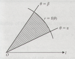
1. For the curve with polar equation r = {\rm f}(\theta), area of shaded region \displaystyle = {1\over 2} \int_\alpha^\beta r^2 {\rm d}\theta = {1\over 2} \int_\alpha^\beta [{\rm f}(\theta)]^2 {\rm d}\theta
   
   
   
   
2. For tangents parallel to \displaystyle l, {{\rm d}\over {\rm d}\theta}(r\sin \theta) = 0
   
   For tangents perpendicular to \displaystyle l, {{\rm d}\over {\rm d}\theta}(r\cos \theta) = 0