FP3 summary

Chapter 1 summary - Maclaurin and Taylor series

1. If y={\rm f}(x) , successive differentiation with respect to x gives:
   
   \displaystyle {{\rm d}y\over {\rm d}x} = {\rm f}'(x), {{\rm d}^2y\over {\rm d}x^2} = {\rm f}''(x), ... , {{\rm d}^ny\over {\rm d}x^n} = {\rm f}^{(n)}(x)
   
   
2. Maclaurin's expansion:
   
   \displaystyle {\rm f}(x) = {\rm f}(0) + {x\over 1!}{\rm f}'(0) + {x^2\over 2!}{\rm f}''(0) + ... + {x^r\over r!}{\rm f}^{(r)}(0) + ...
   
   
3. \displaystyle \sin x = x - {x^3\over 3!} + {x^5\over 5!} - ... + (-1)^r{x^{2r+1}\over (2r+1)!}+ ...
   
   
4. \displaystyle \cos x = 1 - {x^2\over 2!} + {x^4\over 4!} - ... + (-1)^r{x^{2r}\over (2r)!}+ ...
   
   
5. \displaystyle \ln (1+x) = x - {x^2\over 2!} + {x^3\over 3!} - ... + (-1)^{r+1}{x^r\over r!}+ ...
   
   
6. \displaystyle {\rm e}^x = 1 + x + {x^2\over 2!} + {x^3\over 3!} - ... + {x^r\over r!} + ...
   
   

For sufficiently small x , where x^3 and higher powers of x are disregarded:


7. \displaystyle \sin x \approx x \approx \tan x
   
   
8. \displaystyle \cos x \approx 1 - {1\over 2}x^2
   
   
9. \displaystyle (1+x)^{1\over 2} \approx 1 + {1\over 2}x - {1\over 8}x^2
   
   
10. \displaystyle \ln(1+x) \approx x - {1\over 2}x^2
    
    
11. \displaystyle {\rm e}^x \approx 1 + x + {1\over 2}x^2
    
    
12. Taylor's series for {\rm f}(x+a) in ascending powers of x is
    
    \displaystyle {\rm f}(x+a) = {\rm f}(a) + x{\rm f}'(a) + {x^2\over 2!}{\rm f}''(a) + ... + {x^r\over r!}{\rm f}^{(r)}(a) + ...
    
    where a is a constant.
    
    
13. Taylor's series for {\rm f}(x) in ascending powers of (x -a) is
    
    \displaystyle {\rm f}(x) = {\rm f}(a) + (x-a){\rm f}'(a) + {(x-a)^2\over 2!}{\rm f}''(a)+...+ {(x-a)^r\over r!}{\rm f}^{(r)}(a)+...
    
    where a is a constant.
    
    
14. The Taylor series solution of the differential equation \displaystyle {dy\over dx} = {\rm f}(x,y) for which y = y_0 at x = x_0 is
    
    \displaystyle y = y_0 + (x - x_0)\left({{\rm d}y\over {\rm d}x}\right)_{x_0} + {(x - x_0)^{2}\over 2!}\left({{\rm d}^2y\over {\rm d}x^2}\right)_{x_0} + {(x - x_0)^{3}\over 3!}\left({{\rm d}^3y\over {\rm d}x^3}\right)_{x_0} + ...
    
    where \displaystyle \left({{\rm d}^ny\over {\rm d}x^n}\right)_{x_0} is the value of \displaystyle {{\rm d}^ny\over {\rm d}x^n} at x = x_0 .
    
    Often x_0 = 0 , and the solution is
    
    \displaystyle y = y_0 + x \left({dy\over dx}\right)_0 + {x^2\over 2!}\left({dy\over dx}\right)_0 + {x^3\over 3!}\left({dy\over dx}\right)_0 + ...
    
    
15. An approximate value of a definite integral can sometimes be found by expanding the integrand in a series and then integrating the series term by term. This only works satisfactorily when the limits are substituted, if successive terms after the first few are rapidly getting smaller and smaller.

Chapter 2 summary - Complex numbers

1. The complex number z = a + ib, a, b \in \Re can also be written as
   
   z = r(\cos \theta + i\sin \theta) \quad and \quad z = re^{i\theta}
   
   where -\pi < \theta \leq \pi and where r = \sqrt {(a^2 + b^2} and \theta is the angle which the line representing z on an Argand diagram makes with the positive x-axis.
   
   
2. \cos iz = \cosh z
   \sin iz = i\sinh z
   \cosh iz = \cos z
   \sinh iz = i\sin z
   
   where z \in \unicode{x2102} .
   
   
3. If z_1 = r_1(\cos \theta_1 + i\sin\theta_1) and z_2 = r_2(\cos \theta_2 + i\sin\theta_2) then
   
   z_1z_2 = r_1r_2[\cos(\theta_1+\theta_2) + i\sin(\theta_1+\theta_2)]
   \displaystyle {z_1\over z_2} = {r_1\over r_2}[\cos(\theta_1-\theta_2) + i\sin(\theta_1-\theta_2)]
   
   
4. De Moivre's Theorum states that if
   
   z = r(\cos \theta + i\sin \theta)
   
   then
   
   z^n = r^n(\cos n\theta + i\sin n\theta)
   
   
5. The nth roots of unity are such that
   
   
   1. one root is always 1
   2. if n is even, another root is always -1
   3. there are n roots and if these are represented on an Argand diagram then the angle between any two consecutive roots is \displaystyle {2\pi\over n}
   4. the roots can be written as 1, \omega, \omega^2, \omega^3, ..., \omega^{n-2}, \omega^{n-1}
   5. with the exception of 1 (and -1 if n is even) the roots occur in conjugate pairs
   6. 1 + \omega + \omega^2 + \omega^3 + ... + \omega^{n-2} + \omega^{n-1} = 0
   
   
6. |z_1 + z_2| \leq |z_1| + |z_2|
   |z_1 + z_2| \geq \bigl||z_1| - |z_2|\bigr|

Chapter 3 summary - Matrix algebra

1. A linear transformation T is such that
   
   T(a_1{\bf v}_1 + a_2{\bf v}_2) = a_1T({\bf v}_1) + a_2T({\bf v}_2)
   
   where a_1, a_2 are scalars and {\bf v}_1, {\bf v}_2 are vectors.
   
   
2. If T and S are linear transformations then TS is also a linear transformation and
   
   \displaystyle TS({\bf v}) = T[S({\bf v})]
   
   
3. If a linear transformation T is one-one then an inverse linear transformation T^{-1} exists.
   
   
4. Matrix multiplication is not commutative. That is, in general,
   
   {\bf A B} \not= {\bf B A}
   
   
5. The 2 × 2 identity matrix is \displaystyle {\bf I} = \pmatrix{1& 0\\ 0& 1}
   
   The 3 × 3 identity matrix is \displaystyle {\bf I} = \pmatrix{1& 0& 0\\ 0& 1& 0\\ 0& 0& 1}
   
   
6. {\bf AB} = {\bf I} , then {\bf B} = {\bf A}^{-1} and {\bf A} = {\bf B}^{-1} .
   
   
7. \displaystyle {\bf I} = \pmatrix{p& q\\ r& s} = {1\over ps-qr} \pmatrix{s& -q\\ -r& p}
   
   
8. If \displaystyle {\bf A} = \pmatrix{a& b& c\\ d& e& f\\ g& h& i} then the transpose of {\bf A} is
   
   \displaystyle {\bf A}^{\rm T} = \pmatrix{a& d& g\\ b& e& h\\ c& f& i}
   
   
9. Det \displaystyle {\bf A} = \left|\matrix{a& b& c\\ d& e& f\\ g& h& i}\right| = a\left|\matrix{e& f\\ h& i}\right| - b\left|\matrix{d& f\\ g& i}\right| + c\left|\matrix{d& e\\ g& h}\right|
   
   
10. To find the inverse of a 3 × 3 matrix you
    
    
    1. form the matrix of minors
    2. form the matrix of cofactors
    3. transpose the matrix of cofactors
    4. divide the matrix of cofactors by the determinant.
    
    
11. A matrix is called singular if its determinant is zero.
    
    
12. Only non-singular square matrices have an inverse.
    
    
13. To find a 3 × 3 matrix which represents a linear transformation T, you find T({\bf i}) , T({\bf j}) and T({\bf k}) and make these the first, second and third columns respectively of the matrix.
    
    
14. If {\bf A} and {\bf B} are two matrices then
    
    \displaystyle ({\bf AB})^{-1} = {\bf B}^{-1}{\bf A}^{-1}
    \displaystyle ({\bf AB})^{\rm T} = {\bf B}^{\rm T}{\bf A}^{\rm T}
    
    
15. If {\bf A} is a matrix and {\bf v} is a non-zero vector such that {\bf Av} = \lambda{\bf v} where \lambda is a scalar, then {\bf v} is called an eigenvector of {\bf A} and \lambda is the corresponding eigenvalue.
    
    
16. |{\bf A} - \lambda{\bf I}| = 0 is the characteristic equation of the matrix {\bf A}. The solutions of this equation given the eigenvalues of {\bf A}.
    
    
17. \displaystyle {1\over \sqrt {(a^2+b^2+c^2)}} \pmatrix{a\\ b\\ c} is the normalised eigenvector of \pmatrix{a\\ b\\ c} .
    
    
18. The eigenvectors {\bf v}_1 and {\bf v}_2 are orthogonal if
    
    {\bf v}_1 \cdot {\bf v}_2 = 0
    
    
19. The matrix \displaystyle \pmatrix{a& b& c\\ d& e& f\\ g& h& i} is orthogonal if \pmatrix{a\\ d\\ g} , \pmatrix{b\\ e\\ h} and \pmatrix{c\\ f\\ i} are each normalised eigenvectors and if \pmatrix{a\\ d\\ g} \cdot \pmatrix{b\\ e\\ h} = 0 , \pmatrix{a\\ d\\ g} \cdot \pmatrix{c\\ f\\ i} = 0 and \pmatrix{b\\ e\\ h} \cdot \pmatrix{c\\ f\\ i} = 0 .
    
    
20. If {\bf A} is orthogonal then {\bf A}^{\rm T} = {\bf A}^{-1} .
    
    
21. A square matrix whose elements are all zero except those on the leading diagonal is called a diagonal matrix.
    
    \displaystyle \pmatrix{a& 0\\ 0& b} and \displaystyle \pmatrix{a& 0& 0\\ 0& b& 0\\ 0& 0& c} are diagonal matrices.
    
    
22. A matrix {\bf A} which has {\bf A}^{\rm T} = {\bf A} is symmetric.
    
    
23. If {\bf A} is symmetric and {\bf P} is an orthogonal matrix whose columns are the normalised, orthogonal eigenvectors of {\bf A}, then {\bf P}^{\rm T}{\bf AP} is diagonal.

Chapter 4 summary - Vectors

1. The vector product of {\bf a} and {\bf b} is
   
   {\bf a} \times {\bf b} = |{\bf a}||{\bf b}|\sin \theta \hat {\bf n}
   
   where \theta is the angle between {\bf a} and {\bf b} and \hat {\bf n} is a unit vector perpendicular to both {\bf a} and {\bf b} which is in the direction that a right-handed corkscrew would move when turned from {\bf a} to {\bf b}.
   
   
2. {\bf a} \times {\bf b} = -{\bf b} \times {\bf a}
   
   
3. 1. {\bf i} \times {\bf j} = {\bf k}
   2. {\bf j} \times {\bf k} = {\bf i}
   3. {\bf k} \times {\bf i} = {\bf j}
   
   where {\bf i}, {\bf j}, {\bf k} are the unit vectors in the directions of the positive x-, y- and z-axes respectively.
   
   
4. 1. {\bf i} \times {\bf i} = {\bf 0}
   2. {\bf j} \times {\bf j} = {\bf 0}
   3. {\bf k} \times {\bf k} = {\bf 0}
   
   where {\bf i}, {\bf j}, {\bf k} are the unit vectors in the directions of the positive x-, y- and z-axes respectively.
   
   
5. If {\bf a} = a_1{\bf i} + a_2{\bf j} + a_3{\bf k}
   and {\bf b} = b_1{\bf i} + b_2{\bf j} + b_3{\bf k}
   
   then {\bf a} \times {\bf b} = \left|\matrix{{\bf i}& {\bf j}& {\bf k}\\ a_1& a_2& a_3\\ b_1& b_2& b_3}\right|
   
   
6. If {\bf a} \times {\bf b} = {\bf 0} then either {\bf a} = {\bf 0} or {\bf b} = {\bf 0} or {\bf a} and {\bf a} are parallel.
   
   
7. 
   
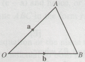
   Area of \triangle AOB = {1\over 2}|{\bf a} \times {\bf b}|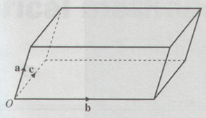
   
   
8. 
   
   The volume of the parallelepiped is
   
   {\bf a} \cdot {\bf b} \times {\bf c}
   
   
9. If {\bf a} = a_1{\bf i} + a_2{\bf j} + a_3{\bf k}
   {\bf b} = b_1{\bf i} + b_2{\bf j} + b_3{\bf k}
   {\bf c} = c_1{\bf i} + c_2{\bf j} + c_3{\bf k}
   
   then {\bf a} \cdot {\bf b} \times {\bf c} = \left|\matrix{a_1& a_2& a_3\\ b_1& b_2& b_3\\ c_1& c_2& c_3}\right| .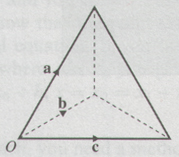
   
   
10. 
    
    The volume of the tetrahedron is
    
    {1\over 6}{\bf a} \cdot {\bf b} \times {\bf c}
    
    
11. The equation of the line passing through A, with position vector {\bf a}, and the point R, with position vector {\bf r}, and which is parallel to the vector {\bf b}, is
    
    ({\bf r} - {\bf a}) \times {\bf b} = {\bf 0}
    
    
12. The equation of the plane containing the points A and R, with position vectors {\bf a} and {\bf r} respectively, is {\bf r} \cdot {\bf n} = p , where p = {\bf a} \cdot {\bf n} and {\bf n} is a vector perpendicular to the plane.
    
    
13. The vector equation of a plane passing through the point with position vector {\bf a} and where {\bf b} and {\bf c} are non-parallel vectors in the plane, neither of which is zero is
    
    {\bf r} = {\bf a} + \lambda{\bf b} + \mu{\bf c} ,
    
    where \lambda and \mu are scalars.
    
    
14. The distance d from the origin to the plane containing the point with position vector {\bf r} is
    
    d = {\bf r} \cdot \hat {\bf n}
    
    where \hat {\bf n} is a unit vector perpendicular to the plane.
    
    
15. The acute angle \theta between a line, with direction vector {\bf b}, and a plane is
    
    \displaystyle \arcsin \left|{{\bf b}\cdot{\bf n}\over |{\bf b}||{\bf n}|}\right|
    
    where {\bf n} is a vector perpendicular to the plane.
    
    
16. The acute angle \theta between two planes is given by
    
    \displaystyle \cos \theta = \left|{{\bf n}_1\cdot{\bf n}_2\over |{\bf n}_1||{\bf n}_2|}\right|
    
    where {\bf n}_1 is a vector perpendicular to one of the planes and {\bf n}_2 is a vector perpendicular to the other plane.
    
    
17. The shortest distance between the lines with equations {\bf r} = {\bf a} + \lambda{\bf b} and {\bf r} = {\bf c} + \mu{\bf d} where \lambda, \mu are scalars is given by
    
    \displaystyle \left|{({\bf a} - {\bf c})\cdot{\bf b}\times{\bf d}\over |{\bf b}\times{\bf d}|}\right|

Chapter 5 summary - Numerical methods

1. In step-by-step methods, where the step length is h, learn the approximations and how to use them:
   
   \displaystyle \left({dy\over dx}\right)_0 \approx {y_1-y_0\over h}
   \displaystyle \left({dy\over dx}\right)_0 \approx {y_1-y_{-1}\over 2h}
   \displaystyle \left({d^2y\over dx^2}\right)_0 \approx {y_1-2y_0+y_{-1}\over h^2}

Chapter 6 summary - Proof